### Transformation
## Parameters
# circle_x is x value of center
# circle_y is y value of center
# circle_radius is radius
# point_1 is one point from 0 to 2*pi
# point_2 is one point from 0 to 2*pi
## Returns
# dataframe with
# point_1_x, point_1_y, point_2_x, point_2_y, midpoint_x, midpoint_y
line_points <- function(circle_x, circle_y, circle_radius, point_1, point_2) {
# Get x,y values
point_1_x = circle_x + circle_r * cos(point_1)
point_1_y = circle_y + circle_r * sin(point_1)
point_2_x = circle_x + circle_r * cos(point_2)
point_2_y = circle_y + circle_r * sin(point_2)
# Get midpoints
midpoint_x = (point_1_x + point_2_x) / 2
midpoint_y = (point_1_y + point_2_y) / 2
return(data.frame(point_1_x = point_1_x,
point_1_y = point_1_y,
point_2_x = point_2_x,
point_2_y = point_2_y,
midpoint_x = midpoint_x,
midpoint_y = midpoint_y))
}
##-------------
# Dataset setup
##-------------
lines <- data.frame(line = seq(1, n_lines),
point_1 = runif(n_lines, 0, 2 * pi),
point_2 = runif(n_lines, 0, 2 * pi))
lines <- lines %>%
bind_cols(pmap_dfr(list(circle_x = circle_h,
circle_y = circle_k,
circle_radius = circle_r,
point_1 = .$point_1,
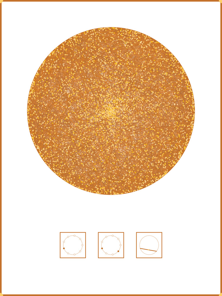
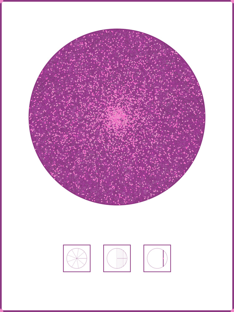
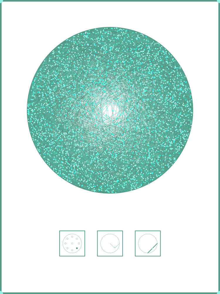
point_2 = .$point_2), line_points))This project is based on the Bertrand Paradox. The Bertrand Paradox deals with patterns that develop from sampling points/chords in a circle. The paradox occurs when different sampling methods seem like they should have the same output but don’t. The first method for this project samples two points on the perimeter then connects them to get the line and the midpoint to get the point. The second method samples a radius at a random angle around the circle, then a random distance on that radius for the midpoint. The line at a right angle is the chord. The last method samples a random point at uniform in the circle for the midpoint. Then the line at a right angle to the segment from that point to the center is the chord. Each of these produces a different distribution of lines and points.
The code can be found here. We’ll walk through a subset of it in this post. For each method, we generate some features at random, then get lines and points from them.
Randomization Methods
For these methods, we’ll build a function called line_points that takes in the center and radius of the circle along with the features we randomly generated for each method. The function outputs the two endpoints for the chord and the midpoint. After creating line_points, we’ll generate the random features then run them through pmap_dfr from the purrr package to apply the line_points function.
For the following code snippets, circle_h, circle_k, and circle_radius are the circle’s center x coordinate, center y coordinates, and radius.
For method 1, we generate the two points on the perimeter as uniform distances from 0 to 2 * pi. Then we take each of those and convert them to coordinates based on the circle’s center and radius. Finally, get the midpoint and return.
For method 2, our line_points function needs a radius (random uniform from 0 to 2 * pi) and the proportionate distance from the center to the perimeter (random uniform from 0 to 1). The line_points function takes those values, converts the proportion to the actual distance, finds the ends of a chord crossing that point if the angle was 0, rotates everything to the appropriate angle, then moves to the circle’s location.
### Transformation
## Parameters
# circle_x is x value of center
# circle_y is y value of center
# circle_radius is radius
# radius is radian
# chord is fraction along the radius
## Returns
# dataframe with
# point_1_x, point_1_y, point_2_x, point_2_y, midpoint_x, midpoint_y
line_points <- function(circle_x, circle_y, circle_radius, radius, chord) {
  # move out to radius from origin
  x_1 = circle_radius * cos(radius)
  y_1 = circle_radius * sin(radius)
  x_2 = circle_radius * cos(radius)
  y_2 = circle_radius * sin(radius)

  # https://www.mathsisfun.com/algebra/trig-solving-ssa-triangles.html
  # we know one angle is 90*
  # one side is circle_radius
  # one side is chord
  new_angle = pi - pi/2 - asin(((chord * circle_radius) *
                                  sin(pi/2)) / circle_radius)

  # now rotate these points around to the radius
  x_1_moved = cos(new_angle) * x_1 - sin(new_angle) * y_1
  y_1_moved = sin(new_angle) * x_1 + cos(new_angle) * y_1
  x_2_moved = cos(-new_angle) * x_2 - sin(-new_angle) * y_2
  y_2_moved = sin(-new_angle) * x_2 + cos(-new_angle) * y_2

  # move back to where the circle is
  x_1_moved = x_1_moved + circle_x
  y_1_moved = y_1_moved + circle_y
  x_2_moved = x_2_moved + circle_x
  y_2_moved = y_2_moved + circle_y

  return(data.frame(point_1_x = x_1_moved,
                    point_1_y = y_1_moved,
                    point_2_x = x_2_moved,
                    point_2_y = y_2_moved,
                    midpoint_x = (x_1_moved + x_2_moved) / 2,
                    midpoint_y = (y_1_moved + y_2_moved) / 2))
}

##-------------
# Dataset setup
##-------------
lines <- data.frame(line = seq(1, n_lines),
                    radius = runif(n_lines, 0, 2*pi),
                    chord = runif(n_lines, 0, 1))
lines <- lines %>%
  bind_cols(pmap_dfr(list(circle_x = circle_h,
                          circle_y = circle_k,
                          circle_radius = circle_r,
                          radius = .$radius,
                          chord = .$chord), line_points))
For method 3, line_points now needs a point’s x and y coordinates in the unit circle. We then find the chord by rotating the point to angle 0 then finding the vertical line through that point. The chord’s endpoints are where the vertical line crosses the circle. We then rotate those points back, so their midpoint matches the original point.
### Transformation
## Parameters
# circle_x is x value of center
# circle_y is y value of center
# circle_radius is radius
# point_x is the x value of the random point
# point_y is the y value of the random point
## Returns
# dataframe with
# point_1_x, point_1_y, point_2_x, point_2_y, midpoint_x, midpoint_y
line_points <- function(circle_x, circle_y, circle_radius, point_x, point_y) {
  # move out to radius from origin
  point_x = circle_radius * point_x
  point_y = circle_radius * point_y

  # rotate so just dealing with y
  flatten_by = atan2(point_y, point_x)

  # now rotate these points around to the radius
  x_rotated = cos(-flatten_by) * point_x - sin(-flatten_by) * point_y
  y_rotated = sin(-flatten_by) * point_x + cos(-flatten_by) * point_y # Should be zero

  # find y values
  # x^2 + y^2 = r^2
  # y^2 = r^2 - x^2
  # y = +/- sqrt(r^2 - x^2)
  y1 = sqrt(circle_radius^2 - x_rotated^2)
  y2 = -sqrt(circle_radius^2 - x_rotated^2)

  # rotate back
  point_1_x = cos(flatten_by) * x_rotated - sin(flatten_by) * y1
  point_1_y = sin(flatten_by) * x_rotated + cos(flatten_by) * y1
  point_2_x = cos(flatten_by) * x_rotated - sin(flatten_by) * y2
  point_2_y = sin(flatten_by) * x_rotated + cos(flatten_by) * y2

  # move back to where the circle is
  point_1_x = point_1_x + circle_x
  point_1_y = point_1_y + circle_y
  point_2_x = point_2_x + circle_x
  point_2_y = point_2_y + circle_y

  return(data.frame(point_1_x = point_1_x,
                    point_1_y = point_1_y,
                    point_2_x = point_2_x,
                    point_2_y = point_2_y,
                    midpoint_x = (point_1_x + point_2_x) / 2,
                    midpoint_y = (point_1_y + point_2_y) / 2))
}

##-------------
# Dataset setup
##-------------
lines <- data.frame(line = seq(1, n_lines),
                    r = sqrt(runif(n_lines, 0, 1)),
                    theta = runif(n_lines, 0, 2*pi))
lines <- lines %>%
  mutate(point_x = r * cos(theta),
         point_y = r * sin(theta)) %>%
  select(line, point_x, point_y)
lines <- lines %>%
  bind_cols(pmap_dfr(list(circle_x = circle_h,
                          circle_y = circle_k,
                          circle_radius = circle_r,
                          point_x = .$point_x,
                          point_y = .$point_y), line_points))
Now that we have the basic attributes for the three methods, we can talk about coloring them.
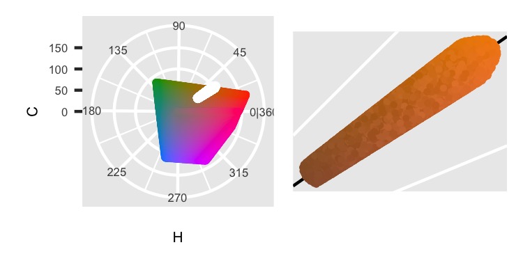
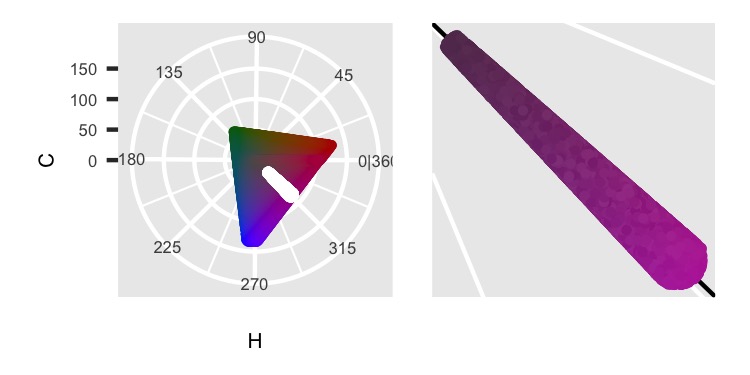
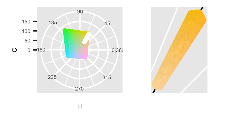
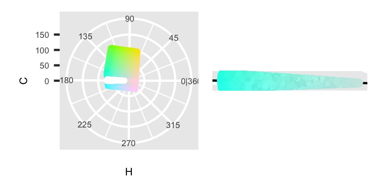
Color Selection
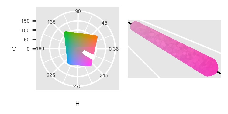
For the methods, I wanted each one to be colored based on different hues. So, I selected them from a yellow-orange/blue-green/purple-red triad. The colors are sampled from ellipses in the HCL color space. The following images show samples from the same ellipses. The line colors are on top and points on the bottom.
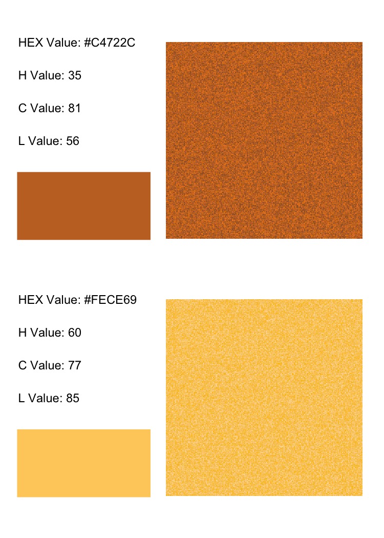
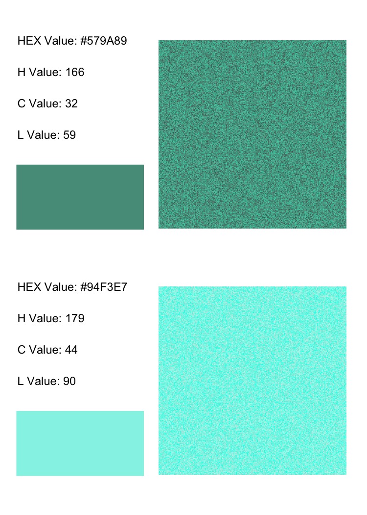
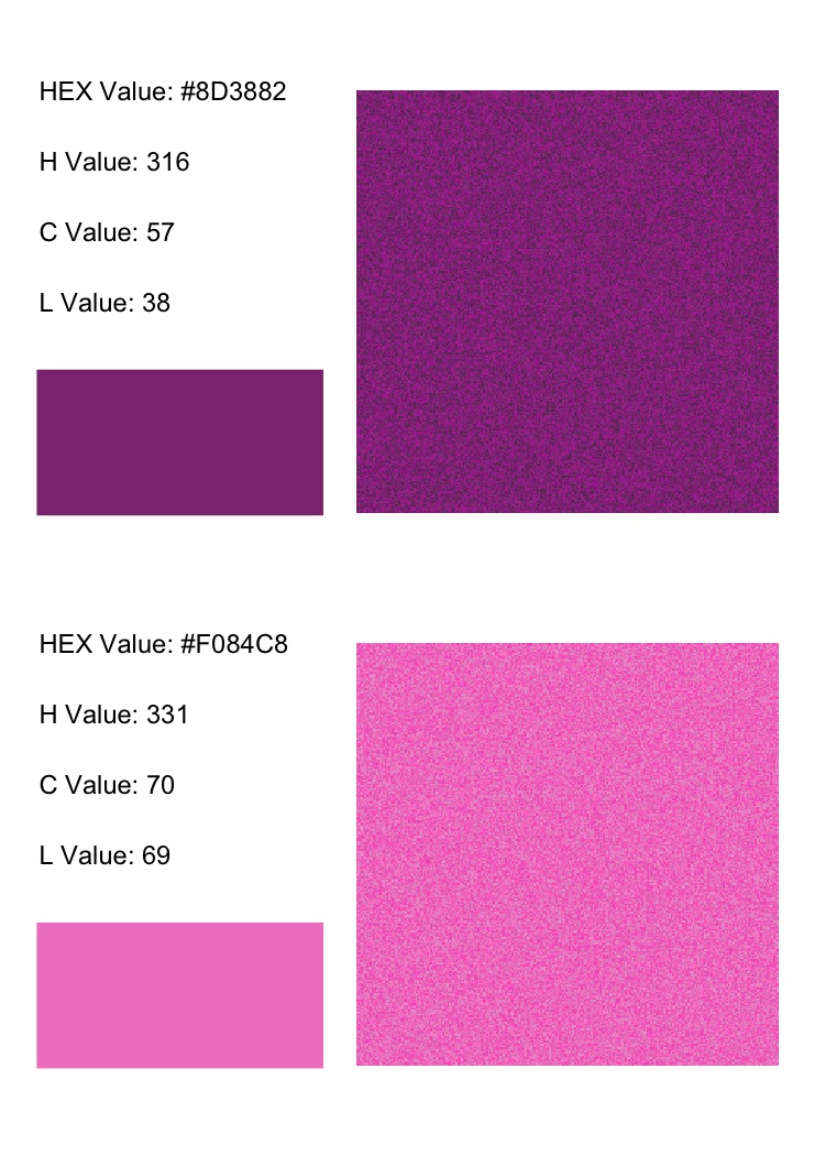
In addition to the lines having a lower base Luminance value, the lines’ ellipses are tilted down towards the center while the points’ slope upwards on the Chroma-Luminance plane for their respective Hue values.
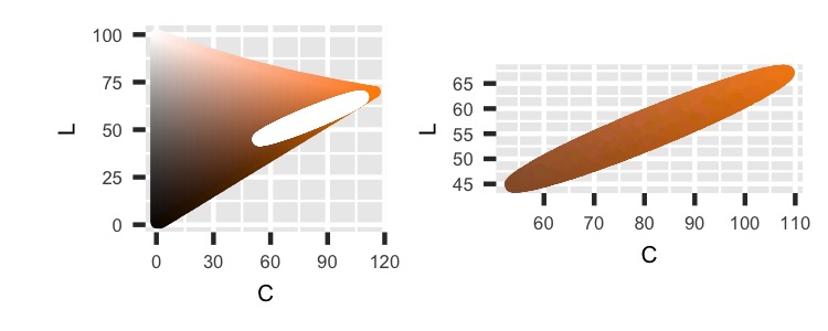
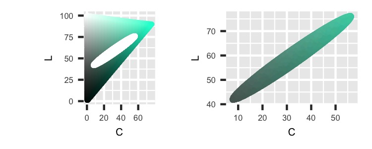
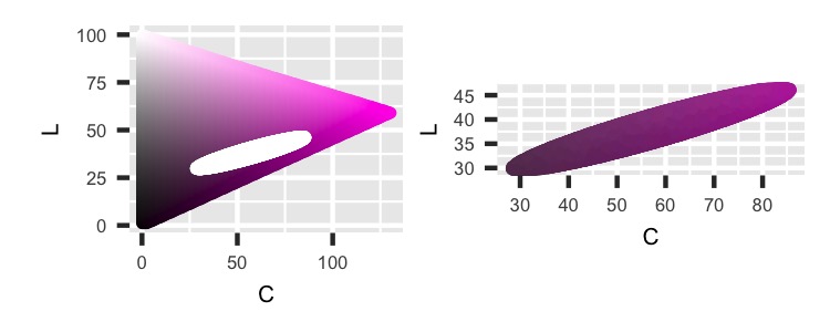
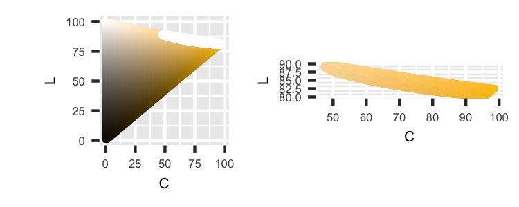
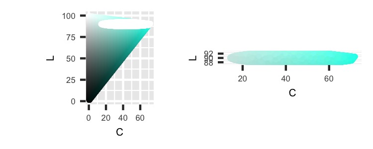
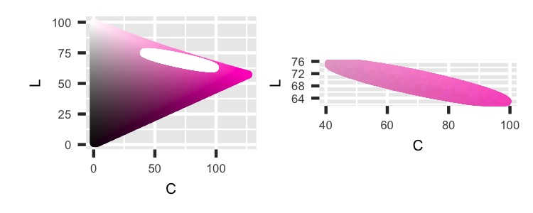
Each of the lines is closer to the secondary colors in Hue than the points. For the order, the revolve around the color wheel counter-clockwise. We can see this when looking at the Hue-Chroma plane at their respective Luminance values.

I tried picking the colors by algorithm, but I couldn’t get that to work as well as I wanted. I often ended up with too much brown or blue. So, the base colors are hand-picked.
Final Output
Now that we can generate the lines/point and colors let’s stick it together. We’ll add diagrams towards the bottom of the images to explain the methods along with borders. The Github repo contains the complete code if you want to see it. The diagrams are affected by the random seed, so any example lines/points can be chosen. I used grid for this instead of ggplot2 because I wanted the points and lines to overlap back and forth. That was easier to do with grid. Later I changed and put all the points on top of all the lines, but by then, I had it all done in grid. I also found this setup easier to control where to place everything on the page instead of worrying about margins or other artifacts getting in the way.
From here to the end are the final products. Better 18” x 24” jpeg files can be found here.